A formalism to describe token systems

The Web3 has given many financial terms an expanded meaning that can lead to misunderstandings. To counter this, this article elaborates a precise formalization using the fundamental functionalities of blockchains and tokens based on the ERC20 . This standard describes the most widely used functionalities of blockchains for fungible tokens:

• ERC20.symbol() returns the symbol of the token das Symbol des Tokens aus.
• ERC20.balanceOf(address) returns the balance of the given address
• ERC20.transfer(receiver, amount) transfers the given amount of token from the address of the caller to the receiver address.
• ERC20.totalSupply() returns the total supply of the token.

Notational conventions

The notation introduced here is based on 4 indices that can be placed at different positions. Both left and right upper and lower indices are used. The resulting object thus consists of 5 components, $\;_\square^\square\Box_\square^\square$ and is to be understood as a whole as a placeholder for a single number.

Tokens, user and address

Als synonym betrachten wir:

• Token symbol and Token address, e.g. DAI and 0x6b175474e89094c44da98b954eedeac495271d0f . These are specified as lower or upper right indexes with lower case Latin letters ("$i$").
• Users, addresses associated with them, and addresses of non-token-generating smart contracts (e.g., "pools"). These are specified as lower or upper left indices with lower case Greek letters ("$\alpha$").

Account balances

Account balances always refer to a token $i$, a user $\alpha$, and the block time $t$ and are written as:

$\;^\alpha A_i[t]$

This denotes the balance of token $i$ of the user $\alpha$ at time $t$. It corresponds to a call to the function ERC20(i).balanceOf(alpha), where alpha equals $\alpha$. The capital letter "A" represents arbitrary asset or variable types. If explicit specification of the type is required, it can be replaced by:

• "N" for natural numbers (Integers).
• "R" for real numbers (Decimals).
• "B" for Booleans (True/False).

If already evident from the context, block time and indexes may be omitted or an explicit token or user may be written out: If we consider a uniswap pool with integer account balances for MATIC and DAI, we write the two relevant account balances of the pool as $\;^\text{Uni} N_\text{DAI}$ and $\;^\text{Uni} N_\text{MATIC}$.

Transfers and state-transitions

Transfers, creation ("minting"), and destruction ("burning") of tokens condition state transitions, which we conceive as a sequence of time-dependent account balances:

$\;^\alpha A_i[0] \rightarrow \;^\alpha A_i[1] \rightarrow ... \;^\alpha A_i[t] \rightarrow \;^\alpha A_i[t+1] $

The single state transition can be written in a shortened form by omitting the time variable $t$ and instead marking the new state with a dash:

$\;^\alpha A_i \rightarrow \;^\alpha A_i' $

For a token transfer two account balances have to be modified: The sender's account balance $\alpha$ is reduced by the amount $M$ to be transferred and the recipient's account balance $\beta$ is increased by the same amount:

$\;^\alpha A_i' = \;^\alpha A_i - M $

$\;^\beta A_i' = \;^\beta A_i + M$

In order to uniquely and unmistakably write which state is modified how, we introduce a $\Delta$ that precedes the changing state. Therefore, for the previously written state changes the following applies:

$ \Delta \;^\alpha A_i' = - M $

$ \Delta \;^\beta A_i' = M$

Assuming that the total amount of a considered token is conserved, every token disappearing at one address must appear at another so that so sender and receiver are always defined. To write this explicitly, we add the receiver explicitly as a lower index $\Delta\;^\alpha_\beta A_i$. It holds that:

$\Delta\;^\alpha_\beta A_i = -\Delta\;^\beta_\alpha A_i = -M$

This summarizes the two account balance changes of a transfer and we speak of a flow of the token $i$ from $\alpha$ to $\beta$. As a mnemonic, you can imagine a right angle starting at the index of the transferred token, running left to the sender address, and then pointing up to the receiver address: $\uparrow\underleftarrow{\Delta\;^\alpha_\beta A_i}$.

Token flows and also more general state transitions are implemented on Etthereum-like blockchains as functions of a smart contracts and thus usually associated with a token. Our notation is illustrated by the example of the transfer function of DAI, which transfers the token amount $M$ from $\alpha$ to $\beta$, where the sender is also explicitly specified:

$\text{DAI.transfer}(\alpha, \beta, M)\{$

$\;^\alpha A_\text{DAI}' = \;^\alpha A_\text{DAI} - M;$

$\;^\beta A_\text{DAI}' = \;^\beta A_\text{DAI} + M;$

$\} $

Written more compactly:

$\text{DAI.transfer}(\alpha, \beta, M)\{$

$\Delta^\alpha_\beta A_\text{DAI} = -M;$

$\} $

We first list the Relevant Token to which the function is assigned. This is followed by a dot after which the functions name is written. In round brackets the parameters and in curved brackets the state transition are given: address.function(parameter){statechanges} Here the state transition can be defined via listings of the form "A' = f(A, ...)" or the deltas. The function "f(A,...)" is called transition function: It takes the "old" variables and calculates a "new" variable from each of them. Alternatively, the so-called invariance, discussed later, can be specified.

Minting/Burning and total supply

Minting and burning of tokens can be understood as transfers from or to a zero address: Minting of tokens at address $\alpha$ corresponds to a positive $\Delta\;^\alpha_0 A_i$ and burning to a positive $\Delta\;^0_\alpha A_i$. We write the total supply of a given token $i$ as "$-\;^{0} A_i$", which corresponds to ERC20(i).totalSupply(). That is, we assume that the zero address has a negative account balance equal to the sum of all other account balances. Thus, it holds:

$\underbrace{\sum_{\alpha \neq 0} \; \;^\alpha A_i}_{\begin{array}{l}\text{sum of all balances}\\\text{except zero address}\end{array}} + \overbrace{\;^{0} A_i}^\text{balance of the zero address} = \underbrace{\sum_{\alpha} \; \;^\alpha A_i}_{\begin{array}{l}\text{sum of all balances}\\\text{including zero address}\end{array}} = 0$

In the first sum, all account balances are added up, excluding the zero address, which is added up separately. The sum on the right side comprises all account balances including that of the zero address. It can be noted in advance that the above context, i.e. $\sum_{\alpha} \; \;^\alpha A_i = 0$, represents the invariance of minting and burning events as well as transfers.

The price functional

Prices and token movements are correlated. The flow of tokens from one address to an address independent of this address, is in generall compensated by an opposing token flow or resource flow: If tokens $i$ are transferred from $\alpha$ to $\beta$, it can be assumed that a quantity of other tokens of equal value $k$ is transferred from $\beta$ to $\alpha$ as compensation. Accordingly, there is a token $k$ with nonvanishing $\Delta\;^\alpha_\beta A_i$ and the two token flows are proportional to each other. As a proportionality factor, we introduce the price functional $\;_\beta^\alpha p_k^i\;$. It indicates how many tokens $k$ correspond to how many tokens $i$ in a trade between user $\alpha$ and user $\beta$, if the tokens $i$ flow from $\alpha$ to $\alpha$ and the tokens $k$ flow from $\beta$ to $\alpha$: The direction of the trade is relevant and the two coupled flows can be obtained by the following mnemonic:

$\underbrace{\uparrow\underleftarrow{\;_\beta^\alpha p_k^i\;}}_{\text{k from }\beta\text{ to }\alpha}\quad\text{ and }\quad\overbrace{\downarrow\overleftarrow{\;_\beta^\alpha p_k^i\;}}^{\text{i from }\alpha\text{ to }\beta}$

Thus, the price functional corresponds to a coupling of two token flows that compensate each other in terms of value and we write:

$\Delta\;^\alpha_\beta A_k = \;_\beta^\alpha p_k^i\; \Delta\;^\beta_\alpha A_i $

The value of the token $i$ on address $\alpha$ from the point of view of address $\beta$ nominated in token $k$ is denoted by $ \;_\beta^\alpha p_k^i\;$. More pointedly spoken: This denotes how much the car ("$i$") of my neighbor ("$\alpha$") is worth to me ("$\beta$ ") measured in pears ("$k$"). Since the same flows can also be described by $-\Delta\;^\beta_\alpha A_i = -\;_\alpha^\beta p_i^k\; \Delta\;^\alpha_\beta A_i $, swapping upper and lower indices of the price functional corresponds to an inversion:

$ \;_\beta^\alpha p_k^i = \frac{1}{\;_\alpha^\beta p_i^k} $

Observe how upper and lower indices find each other and the price functional conditions an index change in the flows: an upper index of the price functional that encounters an equal lower index in the flow replaces it with the corresponding lower index of the price functional. Similarly, a lower index of the price functional that encounters an equal upper index in the flow replaces it with the corresponding upper index of the price functional. This is relevant in that only account balances of the same token can be compared, but multiplication by the price functional allows conversion. Suppose we want to give the value of a portfolio comprising $A_\text{UNI}$ UNI and $A_\text{MATIC}$ MATIC in DAI (i.e. $), where we obtain the prices from a decentralized marketplace (DEX) such as BAL (Balancer), then the value is given by:

$\text{PortfolioValue =}\; \;_\text{BAL} p_\text{DAI}^\text{UNI} * A_\text{UNI} + \;_\text{BAL} p_\text{DAI}^\text{MATIC} * A_\text{MATIC} $

Here we have omitted the upper left index, since a market price is independent of the address on which the asset under consideration is located: For a pool $\alpha$, the price is in general independent of the particular user, so it holds for all $\gamma$ and $\beta$ that $\;_\alpha^\beta p_k^i\; = \;_\alpha^\gamma p_k^i\;$. In such case the upper left index can be omitted and we write $\;_\alpha p_k^i\;$ for the value of token $i$ nominated in token $k$ based on the prices of the pool at address $\alpha$. This indicates how much of token $k$ you get for a token $i$ from the pool $\alpha$:

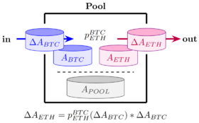
In the figure, $A_\text{POOL}$ denotes the liquidity token of the pool whose value is backed by the amounts $A_\text{BTC}$ and $A_\text{ETH}$ in the pool.

The price functional is formulated in such a general way that it encompasses all common price definitions, but can and must go well beyond them: It is necessary to represent subjective value estimates as well. To do this, we consider the value measured in any asset $i$ that a user $\alpha$ is willing to destroy to create another asset $k$ and write this down as follows:

$ \;_0^\alpha p_k^i$

Thus, we relate subjective value estimation to the price of a token minting: this indicates how much someone is willing to give to obtain a particular good. In contrast, $ \;_\beta^0 p_k^i$ indicates what compensation, measured in $k$, a person $\alpha$ demands to burn an asset $i$. If two subjective value assessments are compatible with each other, an exchange can occur and it holds that $ \;_0^\alpha p_i^k \;_\beta^0 p_i^k = \;_\beta^\alpha p_i^k$.

The price functional is in general not a constant, but may depend, among other things, on $\Delta\;^\alpha_\beta A_i$: $\;_\alpha^\beta p_k^i(\Delta\;^\alpha_\beta A_i)$. This dependence of the price on the tradesize causes that with increasing tradesize one usually gets a worse price. This is called slippage here and will be discussed in more detail later.

Liquidity token

The liquidity token has already been represented in the previous figures as $A_\text{Pool}$, respectively $A_\text{Pool1}$ and $A_\text{Pool1}$ and corresponds to the token issued by the pool, i.e. a stake in the respective pool. We now write the pool's liquidity token as $A_l$ for abbreviation purposes. The share of an address $\alpha$ in the pool $\gamma$ is given by the account balance $\;^\alpha A_l$ of $\alpha$ divided by the total supply $-\;^{0} A_l$, thus:

$\text{Share of }\alpha \quad = \quad -\frac{\;^\alpha A_l}{\;^{0} A_l}$

Liquidity tokens can be obtained in exchange of one or more of those tokens that are contained in the pool (see the left side of the figure below). When they are returned, the tokens contained in the pool are received in the amount of the share corresponding to the liquidity tokens supplied (see the right side of the figure).

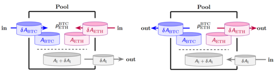
In the transactions considered so far, only two different tokens were involved. This is generalized for liquidity transactions: any number of different tokens can be moved. As a consequence, no unique price can be defined and therefore a generalization of the price functional is necessary, which, however, would go beyond the scope of this article.

The price of the liquidity token is usually collateralized by the value of the pool, with dollar prices used below for simplicity:

$p^\text{l}_\text{\$} \geq \; -\frac{p^\text{BTC}_\text{\$} * \;^\text{Pool} A_\text{BTC} +  p^\text{ETH}_\text{\$} * \;^\text{Pool} A_\text{ETH}}{\;^{0} A_l} $

The negative sign results from the sign of the total supply $-\;^{0} A_l$. This lower bound of the price of a liquidity token is susceptible to impermanent loss, which will be discussed in more detail later.

Important relations

The notation described before allows to describe token systems "statically". The "statics" of a token system can be represented in a single quantity: The invariance of the system.

Invariances

Invariances of a system allow to analyze all possible states of the system at once, which however requires a high mathematical understanding. In this notation, invariances are written with a large calligraphic $\mathcal{I}_\text{state change}$, with the associated state transition as the lower right index. Invariances are quantities that are conserved during state transitions, but are decidedly formed from the changing states. An invariance describes the change of state as comprehensively as transition functions do, which can be determined directly from the invariance. For example, the invariance of a token transfer, i.e., a flow $\Delta\;^\beta_\alpha A_i=M$ is given by $\mathcal{I}_\text{Transfer}=\;^\alpha A_i+\;^\beta A_i$, i.e., the sum of the account states of the sender and receiver addresses. It then holds:

$\mathcal{I}_\text{Transfer}=\;^\alpha A_i+\;^\beta A_i = (\underbrace{\;^\alpha A_i+M}_{\;^\alpha A_i'})+(\underbrace{\;^\beta A_i-M}_{\;^\beta A_i'})=\mathcal{I}'_\text{Transfer}$

The total supply of tokens before the transfer is equal to the total supply after the transfer. In the elaborated formalism this invariance can easily be extended to minting and burning events:

$\mathcal{I}_\text{MintBurnTransfer} = \sum_\alpha \;^\alpha A_i = 0$

Invariance, transition function and price functional are closely related to each other, as explained below using the example of UniSwap:

$\underbrace{\mathcal{I}_\text{Uni}= A_i * A_k}_\text{Invariance} \;\Leftrightarrow\; \underbrace{\Delta A_i = -A_i \frac{\Delta A_k}{A_k+\Delta A_k}}_\text{transition function} \;\Leftrightarrow\; \underbrace{\;^\text{Uni} p_i^k(\Delta A_k) = \frac{ A_i}{A_k+\Delta A_k}}_\text{price functional}$

The transition function results from the following consideration: One changes a variable $A_k \rightarrow A_k' = A_k+\Delta A_k$ to rebalance the resulting change in invariance by changing another variable $A_i \rightarrow A_i' = A_i+\Delta A_i$. This relates one variable change $\Delta A_k$ to another $\Delta A_i$, which directly corresponds to the transition function. The price functional is determinable from the negative ratio of changes, $-\frac{\Delta A_i}{\Delta A_k}$. In the limit transition of vanishing variable changes, it becomes a derivative, which can be expressed via an implicit derivative of the invariance:

$ p_i^k = - \frac{\partial A_i}{\partial A_k} = \frac{\frac{\partial \mathcal{I}}{\partial A_k }}{\frac{\partial \mathcal{I}}{\partial A_i}} $

In the following, we look at the dynamics of the system, i.e. the interactions of prices and token flows, and which regularities underlie them.

Market driving forces

The nature or physics always strives for a minimization of energy. By minimizing an energy functional, a multitude of natural phenomena can be explained and predicted. We are now looking for comparable quantities, the minimization of which a token system strives for, and speak of market driving forces. When the sought quantities are minimized, price differences and token flows condition on each other, preserving invariances. The simplest case is when two individuals $\alpha$ and $\beta$ agree on a trade in which the individuals exchange an asset $i$ for an asset $k$. In the following, we formalize the driving forces of such exchanges:

$\overbrace{\;_\alpha^0 p_k^i > 1}^{\alpha \text{ wants } k \text{ and gives } i} \text{ und } \underbrace{\;_\beta^0 p_i^k > 1}_{\beta \text{ wants } i \text{ and gives } k} \Rightarrow\quad \Delta\;^\alpha_\beta A_i > 0 \text{ und } \Delta\;^\beta_\alpha A_k>0$

A trade occurs when both agree on a price, i.e. each can take the place of "0" with the other. The following identities then apply:

$\;_\alpha^0 p_k^i = \frac{1}{\;_\beta^0 p_i^k} = \;_0^\beta p_k^i=\;_\alpha^\beta p_k^i = \frac{ \Delta\;^\beta_\alpha A_k}{ \Delta\;^\alpha_\beta A_i}$

Thereby, the flows $\Delta\;^\beta_\alpha A_k$ and $\Delta\;^\alpha_\beta A_i$, respectively the price $\;_\alpha^\beta p_k^i$ are realized. These result from the fact that the two individuals place a different value on the assets and both experience a subjective increase in value in the exchange. The Maximum Value Enhancement is reached when $\;_\alpha^0 p_k^i=1$, i.e. when all assets are distributed in such a way that the subjective value assessments have minimal distance to 1, i.e.: $\text{Min}(|\;_\alpha^0 p_k^i-1|)$. The subjective assessments can be captured by stakeholder analyses at least statistically for system-relevant stakeholders.

The connection between price differences and token flows is easier to grasp. If different prices occur in different pools for the same asset, this causes token flows until price alignment occurs. This is called arbitrage: An arbitrageur $\gamma$ looks at the price between two assets $i$ and $k$ at two different pools $\alpha$ and $\beta$ to profit from price differences: buy cheap to sell expensive directly afterwards. Such an arbitrage opportunity is revealed by the following context:

$\;_\gamma^\alpha p_k^i\; * \;_\gamma^\beta p_i^k\; > 1 $

This is illustrated below using the example of BTC and ETH: arbitrage opportunities allow to negotiate profit.

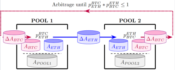
If such a profit opportunity is seized by an arbitrageur $\gamma$, the following token flows are realized: The arbitrageur transfers tokens $k$ to a pool $\beta$, i.e. $\Delta\;^\beta_\gamma A_k > 0$. In return, the arbitrageur receives a corresponding amount of tokens $i$ from the pool, thus, $\Delta\;^\gamma_\beta A_i > 0$. He then swaps in the opposite direction at another pool $\alpha$, corresponding to $\Delta\;^\alpha_\gamma A_i > 0$ and $\Delta\;^\gamma_\alpha A_k > 0$. As such arbitrage opportunities become more likely to be used over time, token systems tend to minimize the following properties:

$\text{Min}(|\;_\gamma^\alpha p_k^i\; * \;_\gamma^\beta p_i^k\;-1|)$

All $\;_\gamma^\alpha p_k^i\; * \;_\gamma^\beta p_i^k$ have a tendency to evolve towards 1.

Arbitrage between two pools usually causes a downward price fluctuation of the liquidity tokens of both pools. The resulting loss in value is called impermanent loss and can be related to the slippage and liquidity of both pools.

In general, it is not possible or only possible with great effort to find the optimal tradesize to achieve maximum profit and direct closing of price gaps (i.e. $\;_\gamma^\alpha p_k^i\; * \;_\gamma^\beta p_i^k$=1 ) with a single arbitrage trade. If the tradesize is too low, the price difference will not be completely eliminated and thus an arbitrage opportunity will still exist. Too high tradesizes overshoot the price gap and open an arbitrage opportunity in opposite direction. Since a large number of arbitrageurs compete for arbitrage opportunities and t "get in each other's way", random price movements are to be expected. Externally driven price changes are therefore expected to overshoot when prices equalize.

The aforementioned market driving forces force the system to gradually converge to the aforementioned minima while preserving invariances. When designing token systems, care must be taken to ensure that they do not exhibit undesirable behavior either along the path to these minima or at the minima themselves. Undesirable behavior can consist, for example, in too high slippage or too high impermanent loss. Minimizing both of these usually represents a conflict of goals.

Slippage

Slippage is the difference between quoted ("spot-price") and realized price and has two causes:

• High volatility, where the price becomes a "moving target" and changes during the trade. Here, the price is not changed due to the trade but independently of it and usually randomly.
• Low liquidity, whereby the price changes with increasing tradesize due to the trade. Here, the trade is the direct cause of the price change and the realized price deteriorates with increasing tradesize.

Slippage relates token flows to price changes and thus also provides a measure of the fragility of the token system: When slippage is high, the system responds with strong price changes to token flows, but with weak token flows to price changes. When slippage is low, the reverse is true. Thus, how the token system reacts to volatility also depends on the slippage.

As the tradesize $\Delta A_k$ increases, there is usually a deterioration in the price of liquidity pools from $p_i^k(0)$ to a $p_i^k(\Delta A_k) \; < \; p_i^k(0)$, so the price change is $p_i^k(\Delta A_k)-p_i^k(0)$. The slippage $s_i^k$ describes how much this deterioration of the price grows with the tradesize $\Delta A_k$.

Impermanent Loss

Impermanent Loss (IL) bezeichnet die Wertminderung eines Liquiditäts-Pools aufgrund einer Preisänderung der im Pool enthaltenen Token: Beim Preisangleich an eine bei anderem Pool erfolgende Preisänderung nimmt ein Pool denjenigen Token auf, der im Preis gefallen ist und gibt denjenigen ab, der im Preis gestiegen ist. Da dies zu den urpsrünglichen Preisen des Pools passiert und nicht zu den sich extern ändernden Preisen, gibt der Pool einen größeren Wert her, als ihm zugeführt wird. Sobald die Preisänderung aber wieder rückgängig gemacht wird, wird auch die Wertminderung wieder ausgeglichen, daher "Impermanent".

IL und Slippage können in einer Vielzahl von Systemen miteinander in Zusammenhang gebracht werden: je größer die Slippage, desto geringere Token-Flüsse sind nötig, um einen Preisangleich zu bewirken und desto geringer ist in der Regel der IL.

Graphtheoretical visualizations

Some of the complexity of the relationships can be hidden by a well-designed graphical representation.

The asset conversion graph

On many token systems arbitrage has great influence and must be well studied. The asset conversion graph allows easy detection of arbitrage cycles.

Each graph $G=(V,E)$ consists of a set of nodes $V$ and a set of edges $E$. For the asset conversion graph, a node is inserted for each relevant token. For each defined price function $\;_\alpha p_i^k$, an edge $\alpha$ is inserted from node $k$ to node $i$. Thus, each edge corresponds to a possible state transition, or swap. Different edges can have the same designation. For a more precise distinction, the designation can be extended by the respective operator: $\alpha.operator(...)$.

For example, consider a system deployed on Polygon in which three different tokens are used: MATIC, DAI and the token of a "TKN" of a system to be developed. The nodes of the graph are thus given by $V=\{MATIC, DAI, TKN\}$. We assume the existence of a UniSwap pool for MATIC and DAI. TKN can be acquired directly at considered system for DAI and resold for MATIC. The corresponding asset conversion graph is given by

$V=\{MATIC, DAI, TKN\} $

$E=\{MATIC\leftrightarrow DAI, DAI\rightarrow TKN, TKN \rightarrow MATIC\} $

and depicted in the following.

An edge weight, illustrated by edge thickness, can be introduced to represent slippage: the lower the slippage, the thicker the edge. The thicker the edge, the more dominant is the operation under consideration in pricing.

It is often relevant who is the price giver and who is the price taker. The edge thickness allows an investigation in this respect: along a given path, the operator with the thickest edge acts as the dominant price giver, operators of thinner edges as price takers.

Possible arbitrage cycles are given by closed paths. For the given graph we can expect arbitrage if

$\;_\text{Uni} p^\text{DAI}_\text{MATIC} < \;_\text{System} p^\text{DAI}_\text{TKN} * \;_\text{System} p^\text{TKN}_\text{MATIC}. $

They are accompanied by the following token flows:

$\Delta\;^\alpha_\text{system} A_\text{DAI}>0 $

$\\ $

$\Delta\;^\text{System}_\alpha A_\text{MATIC}>0$,

where an agent with address $\alpha$ acted as an arbitrageur. From the different edge thicknesses, we can infer that the flow through UniSwap would be larger than the flow through our system under consideration.

In the example given, the system would act as a volatility-driven pump, pumping DAI into the system and MATIC out of the system until no more MATIC is available in the system.

The token flow graph

Total and circulating supply are important variables for token systems: Their evolution depends significantly on how inflationary or deflationary the respective tokens are. Minting and burning events correspond to senders and receivers of tokens.

The token flow graph starts with the insertion of a 0-node, which acts as a source and sink of tokens. For the different tokens specific edge sets are introduced, which can be distinguished from each other by color. Each edge corresponds to an operator that can be invoked by a particular agent. Thus, each edge describes the interaction of an agent with a contract. The nodes of the graph are determined based on possible roles of the agents: each role corresponds to a node.

For previously described system the roles of "trader" is definable. The flow graph of previously described system is shown below.

The figure shows how tokens move through the different subsystems or from agent to agent. For stable systems, any path that starts at the 0 node should return to it. This is satisfied for the depicted graph. Another stability criterion requires that for every edge entering a node, there should be an outgoing edge of the same color. This is not the case for this graph: DAI flows into the system without being able to flow out again and MATIC flows out without being able to flow in.